Remystifying Local weather Suggestions

By Joe Born

1. Introduction

By presenting precise calculation outcomes from a particular feedback-system instance, the plots under will put some graphical meat on the verbal bones of Nick Stokes’ latest “Demystifying Suggestions” publish.

I heartily agree with the principle message I took from Mr. Stokes’ publish: though some local weather equations could also be much like sure equations encountered in, say, electronics, it’s not secure to import electronics outcomes that the local weather equations don’t intrinsically dictate. However I’m much less satisfied that Mr. Stokes succeeded in eradicating the thriller from suggestions. I’m reminded of what a professor stated over a half century in the past in a kind of obligatory science programs: “Don’t simply scope it out; work it out.”

What the professor meant is that we people are likely to overestimate our skills to intuit an equation’s implications. Precise calculations routinely reveal that the equation doesn’t imply what we had thought. That may be true even of equations so simple as the equilibrium scalar suggestions equation at situation right here.

Besides for people who’ve important expertise in working by suggestions techniques, for instance, readers could not take as a lot which means as could be hoped from summary statements reminiscent of the next:

“One factor that’s essential is that you simply hold the units of variables separate. The elements of x0 fulfill a state equation. The perturbation elements fulfill equations, however are proportional to the perturbation. You may’t combine them. That is the essential flaw in Lord Monckton’s latest paper.”

Working by an precise instance may present extra perception. And an event to just do that’s offered by Christopher Monckton’s declare that suggestions principle imposes (what we’ll name) the entire-signal rule:

“[S]uch feedbacks as could subsist in a dynamical system at any given second should perforce reply to your complete reference sign then acquiring, and never merely to some arbitrarily-selected fraction thereof.”

Critics like Mr. Stokes and Roy Spencer have disputed that rule. And, certainly, there are good sensible causes in local weather science for treating suggestions as one thing that’s responsive solely to modifications somewhat than to total portions. But, if we as an alternative settle for Lord Monckton’s entire-signal rule for the sake of argument and work by its implications, we will acquire extra perception into questions like what “you’ll be able to’t combine them” actually means.

So in what follows we’ll settle for that rule and outline an instance suggestions system wherein the suggestions responds to your complete output somewhat than solely to perturbations. And we’ll observe the rule’s implications by working by the system’s responses to a spread of inputs.

Within the course of we’ll juxtapose the small- and large-signal variations of metrics like “suggestions fraction” and “system-gain issue” to disclose the latent ambiguities with which they afflict suggestions discussions. We’ll additionally see examples of how simply the suggestions equation, easy although it’s, may be misinterpreted.

2. Background

First we’ll use the next plot to put Mr. Stokes’ publish in context.

Lord Monckton views the local weather system’s equilibrium temperature

as a perform of the worth it could have if there have been no suggestions. By means of accepting for the sake of argument “all of official climatology besides what we will display to be false,” Lord Monckton has adopted values we’ll name because the equilibrium temperature equivalent to 1850’s carbon-dioxide focus and as what it could have been had there been no suggestions. The purpose labeled “Pre-Industrial” within the plot above represents these values. The purpose labeled “IPCC Prediction” outcomes from growing these values by the “official climatology” ECS worth, , and the worth it could have had with out suggestions. (Equilibrium local weather sensitivity (“ECS”) is the increment by which doubling carbon-dioxide focus would enhance the equilibrium global-mean floor temperature.)

Observational research like Lindzen & Choi 2011 have led many people to imagine that ECS is definitely a lot decrease than that—if there actually is such a factor as ECS. In a video that launched his principle as a “mathematical proof” that ECS is low, although, Lord Monckton stated of earlier ECS-value arguments that that they had “largely been a contest between conjectures.” He could agree with researchers like Lindzen & Choi, he stated, however “they’ll’t completely show that they’re proper.” In distinction, “we predict that what we’ve executed right here is to completely show that we’re proper.”

By in essence projecting these factors to the no-feedback,

line, he finally got here to explain climatology’s error as failing to acknowledge that among the suggestions is response to the emission temperature. And he got here to precise his proof within the type of the above-mentioned entire-signal rule, of which he stated:

“As soon as that time—which is properly established in management principle however has, so far as we will uncover, hitherto solely escaped the eye of climatology—is conceded, because it should be, then it follows that equilibrium sensitivity to doubled CO2 should be low.”

Within the passage quoted above, Mr. Stokes’ publish contested that principle. So we’ve added a hypothetical

curve to the plot for example what high-ECS proponents would possibly assume. However to signify substantial suggestions to the emission temperature the curve passes to the left of the emission-temperature level on the no-feedback, line in compliance with the entire-signal rule.

three. “Underlying Arithmetic”

In a reply to Mr. Stokes’ publish Lord Monckton diagrammed his model

of the equilibrium scalar suggestions equation. That equation appears easy sufficient, however he wrote of its block diagram that “one can solely actually perceive the way it works if one additionally has a grasp of the underlying arithmetic.”

Nevertheless, by treating the (counterfactual) no-feedback temperature

because the enter, Lord Monckton’s equation hides the underlying relationship between the output and forcing. To keep away from the resultant lack of perception we’ll subsequently deal primarily with the forcing relationship, however we’ll map the outcomes to Lord Monckton’s counterfactual-temperature relationship.

For this objective we’ll merely undertake the more-general notation that the system produces a response

to a stimulus ; we received’t attempt to straddle his temperature-input notation and the standard forcing-input notation . If we have been merely to exchange the standard perturbation values with total values, we’d thereby have:

That’s, the output temperature

would merely be the product of a acquire and the sum of the enter forcing and output-dependent suggestions . (The notation for the ratio of suggestions to output shall be to tell apart it from Lord Monckton’s suggestions fraction .) The next express expression for the equilibrium-temperature output would appear to comply with from elementary algebra:

That is all seemingly easy. However even seemingly easy equations may be onerous to interpret. Furthermore, Lord Monckton’s principle requires that we take care of total portions somewhat than simply small perturbations, so we will not ignore nonlinearities.

Subsequently, for the reason that formulation

could recommend that quite the opposite and are constants, we’ll so rewrite the scalar system’s equilibrium equation as explicitly to permit for nonlinearity. Particularly, we’ll exchange with and with :

To map this forcing-input formulation to Lord Monckton’s temperature-input formulation

, we will even calculate a without-feedback temperature , the place denotes ‘s inverse perform: . Lord Monckton’s and respectively correspond to and .

four. Instance-System Capabilities

Now we attain specifics: we’ll outline the capabilities

and in our system equation .

In doing so we received’t try to match the precise local weather relationship between equilibrium temperature and forcing. For one factor, nobody actually is aware of what that relationship is all through your complete area that Lord Monckton would have us acknowledge. To the extent that an equilibrium relationship does exist, furthermore, temperature nearly definitely isn’t a single-valued perform except that perform’s argument is a vector of forcing elements as an alternative of the scalar complete thereof we’re assuming right here. (These problems are among the many explanation why specializing in perturbations is preferable.)

However the query that Lord Monckton’s purported mathematical proof raises isn’t whether or not we all know the connection; it’s whether or not, with out understanding what that relationship is, excessive ECS values may be dominated out mathematically. So we’ll merely select easy relationships that exhibit a excessive ECS worth and look ahead to any contradictions of what Lord Monckton referred to as “the arithmetic of suggestions in all dynamical techniques, together with the local weather.”

four.1 Open-Loop Perform

For our open-loop perform

we undertake a fractional-power relationship:

Word that with

= zero.25 this perform could be a fourth-root relationship harking back to the inverse Stefan-Boltzmann equation. As a nod towards the real-world distinction between the floor temperature and the efficient radiation temperature, nevertheless, we’ve as an alternative adopted , with .

As we see,

‘s slope falls off with enter :

Since

relates an output to an enter, the plot above refers to ‘s slope as a “acquire.” Of explicit significance to this dialogue is that the plot exhibits each the typical slope (large-signal acquire) and the native slope (small-signal acquire). Failure to tell apart between these portions constantly has bedeviled discussions of Lord Monckton’s principle.

Word additionally that we seek advice from each portions as “open-loop acquire”: every is a acquire that the system would exhibit if there have been no suggestions to “shut the loop.” Maybe confusingly—however I believe logically—the dialogue under makes use of comparable expressions to seek advice from totally different portions.

Particularly, closed-loop acquire will seek advice from the acquire that outcomes when suggestions does certainly “shut the loop.” Lord Monckton typically calls this the “system-gain issue.” And simply plain loop acquire would be the inner acquire encountered in traversing the loop: what Lord Monckton often calls the “suggestions fraction.” The loop acquire outcomes from combining the open-loop acquire with the suggestions ratio, which we’ll presently introduce in reference to the suggestions perform.

Once more, the amount to which our open-loop perform

relates the output temperature is forcing. If as Lord Monckton does we as an alternative take the enter to be the no-feedback temperature, the resultant open-loop perform is simply the enter itself: ; if there have been no suggestions, the output could be the identical because the enter.

four.2 Suggestions Perform

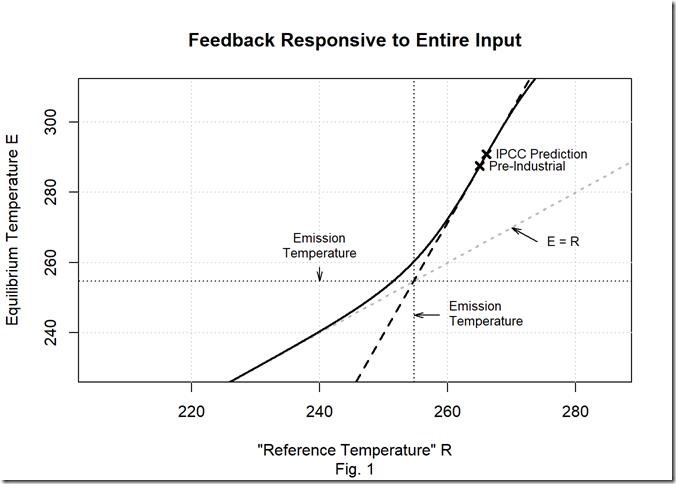
Climatologists typically get media consideration by talking of a “tipping level.” However the explicit suggestions perform we selected for the Fig. 1 curve wouldn’t trigger one. Because the conduct it ends in thereby lacks one among suggestions’s more-interesting options, we’ll as an alternative undertake the next suggestions perform, which causes a tipping level not far past the doubled-CO2 equilibrium temperature:

the place

and

Word that in our feedback-function alternative we differ with Lord Monckton’s critics who object that suggestions can solely be a response to perturbations. Just like the Fig. 1 curve’s suggestions perform, our instance, tipping-point-causing perform is attentive to your complete output. To make certain, the response appears to turn out to be important in each circumstances solely because the temperature approaches ice’s 273 Ok melting level; the response approaches zero because the output temperature does. However really working by the resultant example-system conduct close to absolute zero reveals that due to the excessive ahead acquire we noticed in Fig. three the suggestions is nice sufficient to trigger instability.

Moreover, though the instance perform’s worth on the doubled-CO~2~ temperature approximates that of the suggestions perform answerable for Fig. 1, it exceeds it at temperatures very a lot above or under that temperature. Specifically, our chosen perform’s suggestions to the emission temperature shall be even higher than the Fig. 1 perform’s.

Now, I don’t actually assume both of these suggestions capabilities is just like the precise local weather’s suggestions perform. I personally don’t assume the precise local weather has a lot net-positive suggestions in any respect.

However that’s not the purpose. Lord Monckton claims to have developed a mathematical proof. Meaning displaying that accepting a excessive ECS worth for the sake of argument would result in a contradiction with “the arithmetic of suggestions in all dynamical techniques, together with the local weather.” So the purpose isn’t whether or not we imagine that premise. It’s whether or not accepting the premise leads us to a contradiction. And we’ll search in useless for contradictions among the many implications of a system’s exhibiting not solely a excessive ECS worth but additionally a tipping level.

The plot above exhibits the resultant suggestions ratio, i.e., the amount that multiplies the output or increment thereof to yield our suggestions perform’s corresponding suggestions amount. It’s the suggestions perform’s common (large-signal) slope

or native (small-signal) slope , the place the prime represents differentiation. Once more we see that the large- and small-signal variations differ markedly; one doesn’t approximate the opposite.

Totally different feedback-ratio capabilities, plotted above, consequence if we as an alternative take Lord Monckton’s temperature-input view of the system. These capabilities are common and native slopes of a distinct suggestions perform, of the perform

implied by .

The totally different views’ suggestions ratios are considerably comparable on the greater temperatures we’re curious about, however their low-temperature behaviors are fairly totally different. That doesn’t imply that the temperature-input view is unsuitable. In reality, though I imagine the forcing-input view is often preferable, the temperature-input view would be the more-informative within the case of suggestions ratio, which within the temperature-input view occurs to equal that view’s loop acquire (Lord Monckton’s “suggestions fraction”).

5. Resultant Habits

5.1 Closed-Loop Perform

Having now outlined our system’s open-loop and suggestions capabilities, we flip to the ensuing closed-loop perform, i.e., to the perform

such that our suggestions equation implies :

This plot illustrates the tipping level we so selected our suggestions perform as to trigger. No (equilibrium) output values correspond to enter values that exceed about 273 W/m2. That’s as a result of any greater enter worth would trigger the output to extend with out restrict: the system would by no means attain equilibrium. (If pressed, tipping-point partisans would presumably admit to some restrict, however let’s simply assume their limits are off the chart.) As we’ll see in the end, inputs that exceed the tipping-point enter correspond to a small-signal loop acquire that essentially exceeds unity.

Though the output will increase with out restrict for these values, Lord Monckton says as an alternative (large-signal) “suggestions fraction”

higher than unity would indicate cooling. One can see that it wouldn’t, although, by utilizing Lord Monckton’s personal and for the sake of simplicity assuming a relentless = 1.1 in order that the large- and small-signal values are equal. Beginning with and , iteratively consider . You’ll discover that blows up.

Not like the enter, the output has equilibrium values that exceed its tipping-point worth, which for the output is about 301 Ok. The curve’s dotted portion represents them. The dots point out that the corresponding states are unstable.

You will get an thought of what unstable means by supposing that adverse temperatures have which means in Lord Monckton’s linear

system. Once more assume a relentless = 1.1. If iterations begin at = (1, –10) as an alternative of (1, zero), the output will stay at –10: (1,–10) is certainly an equilibrium state. Nudge the enter someway, although, and in accordance with the route of the nudge the output will take off towards constructive or adverse infinity. Though (zero, –10) is an equilibrium state, that’s, it’s unstable.

The instance system will equally are likely to flee the unstable states and probably blow up. The instance system is nonlinear, although, and the route of the nudge determines whether or not it really does blow up or as an alternative falls to a steady worth, i.e., from the dotted curve to the strong one.

Having seen the output conduct from the forcing-input view, let’s flip to Lord Monckton’s temperature-input view. That’s, let’s think about the perform

such that implies :

This view suppresses the nonlinearity within the relationship between forcing and temperature. Because the enter is solely what the output would have been with out suggestions—whose ratio to output may be very low all through many of the perform’s illustrated area—the output over a lot of the curve almost equals the enter. Towards the fitting, although, the output pulls away. And, simply as within the earlier plot, there’s a tipping level.

5.2 “Suggestions Fraction”

Now we come to what’s maybe the most-consequential amount: the loop acquire, or, in Lord Monckton’s terminology, the “suggestions fraction.” Right here once more we’ll see the significance of distinguishing between large- and small-signal variations.

The plot above confirms what we could have surmised from the earlier plot: the loop acquire is close to zero over many of the perform area. However above-unity loop positive factors on the plot’s proper impose the restrict we noticed on equilibrium-state enter values.

Word specifically that it’s the small-signal model of the loop acquire whose unity worth imposes the restrict; the large-signal loop acquire is kind of modest proper as much as the tipping level. So it’s essential to maintain observe of which amount Lord Monckton intends when he discusses the “suggestions fraction.”

(Obscure technical notice for feedback-theory varieties: Due to the excessive small-signal open-loop acquire close to absolute zero, the system is unstable in that neighborhood despite the fact that the suggestions

approaches zero. For the loop-gain plots we subsequently used adverse inputs to acquire among the near-zero conduct, and to that finish and have been prolonged as odd capabilities into the third quadrant.)

Recall that loop acquire is the acquire encountered in traversing the loop. For the forcing view the large-signal loop-gain model is subsequently the ratio

of the output-temperature-caused suggestions to the entire forcing that induced the output temperature. The small-signal model is the corresponding incremental amount .

Since a unity worth of this dimensionless amount’s small-scale model represents the soundness restrict, one would possibly assume it could be the identical factor in each views. If we really work it out, although, we see there’s a distinction.

For the temperature-input view the large-signal loop-gain amount is the ratio that the suggestions temperature

bears to the output temperature : it’s , which maps to Lord Monckton’s suggestions fraction . The corresponding small-signal model is . On this view the loop acquire is identical because the suggestions ratio we noticed in Fig. 6.

However a comparability of the 2 views’ small-signal loop positive factors is instructive:

Though their small-signal tipping-point values are the identical in each views, the totally different views’ loop positive factors in any other case differ.

5.three “System-Acquire Issue”

We lastly come to closed-loop acquire. This time we’ll begin with Lord Monckton’s temperature-input view. In that view the large-signal model is

. That model corresponds to Lord Monckton’s “system-gain issue” . To calculate ECS’s worth , he advocates multiplying the “reference sensitivity” by that amount.

However by definition the amount whose multiplication by

actually does yield ECS’s appropriate worth is as an alternative the “secant slope” . Even Lord Monckton appears to confess that the secant slope is the fitting multiplier. (Properly, what he really says is, “The drawback of [deriving the “system-gain factor” as a secant slope] just isn’t, repeat not, that it’s unsuitable, however that it isn’t helpful. . . .”) This view’s small-signal acquire corresponds to somewhat than and subsequently equals that secant slope sooner or later within the related interval 265.00 Ok R

Now, in fact his method in all probability wouldn’t end in a severe underestimate if, as many people imagine, ECS is low. That’s as a result of a low worth wouldn’t consequence within the nice between-version distinction that the plot depicts. However that truth doesn’t assist Lord Monckton’s principle.

The issue is that his principle’s targets aren’t individuals who already imagine ECS is low. He characterised his principle as a “approach to compel the assent” of those that would in any other case imagine ECS is excessive. It could compel assent, he stated, as a result of, in contrast to earlier ECS arguments, his principle isn’t a mere conjecture; it’s a proof.

However a proof of low ECS can’t be based mostly on assuming low ECS to start with; that may be begging the query. Nor would the assent of somebody who thinks ECS is excessive be compelled by an method that tremendously underestimates ECS when it’s excessive. What may arguably compel assent is for the high-ECS assumption to end in contradictions of “the arithmetic of suggestions in all dynamical techniques, together with the local weather.” That’s why we took a high-ECS system as our instance: to reveal any such contradictions. However we discovered none.

Now a degree of clarification concerning the plot. The dotted curves principally signify unstable equilibrium states as they did in earlier plots. However right here there’s an exception: the dotted black curve’s vertical phase on the fitting, on the most equilibrium-input worth. That phase is merely the road between positive- and negative-infinity values: its abscissa is the worth at which the closed-loop acquire switches abruptly from constructive to adverse infinity. So no equilibrium states really happen on that vertical phase.

It’d subsequently have been much less distracting to omit that phase from the plot. However it gives one other alternative to level out how onerous it may be to interpret even easy algebraic equations correctly. The corresponding discontinuity within the hyperbola of linear-system acquire ratio as a perform of loop acquire is the premise of Lord Monckton’s above-mentioned perception that loop positive factors higher than unity indicate cooling:

That interpretation is unsuitable, after all; Fig. eight confirmed us that equilibrium output temperature continues to extend past the transition to instability.

Within the electronic-circuit context Lord Monckton has analogously interpreted that discontinuity is as being the purpose “the place the voltage transits from the constructive to the adverse rail.” That interpretation is beguiling due to the viewers’s expertise with audio-system suggestions. In spite of everything, unity loop acquire is the premise for squeal when sound techniques endure from extreme suggestions, and that oscillation definitely includes plenty of voltage “transiting.”

One drawback with such interpretations is that the hyperbola is legitimate just for fixed open-loop acquire. Extra essential, they ignore that the connection represented by the hyperbola is an equilibrium relationship: the hyperbola doesn’t apply to dynamic results like oscillation. (Properly, the equation on which the hyperbola is predicated really can be utilized to characterize steady-state oscillation. However that may require complicated values: the geometric illustration would require 4 dimensions as an alternative of the hyperbola’s two.)

So makes an attempt like Mr. Stokes’ to demystify the suggestions equation itself are all properly and good. However it’s additionally essential to acknowledge that the equation’s very simplicity may be deceptive, even for somebody who “was given coaching within the arithmetic of what are referred to as conic sections.”

Now let’s full our examine of the system’s conduct with the opposite view of closed-loop acquire.

As a substitute of barely growing because the temperature-input view’s large-signal acquire did, the forcing-input view’s really continues to say no proper as much as the tipping level. However the total impact is identical: the small-signal acquire rises dramatically because the tipping level is approached, whereas the large-signal acquire doesn’t.

Briefly, we’ve labored by a counterexample to the proposition that prime ECS values are inconsistent with a system whose suggestions responds to emission temperature. In doing so we’ve detected no contradictions of suggestions arithmetic. However by juxtaposing small- and large-signal variations we’ve seen how essential it’s to tell apart between them constantly.

6. “Close to-Invariant”

Earlier than we conclude, we’ll use one among Lord Monckton’s reactions to such counterexamples for example why it’s essential to “work it out” and never simply “scope it out.”

Ordinarily Lord Monckton’s response to such counterexamples is merely to precise his disbelief that the perform might be so nonlinear. Or he makes the bodily argument that the quasi-exponential response of evaporation to temperature someway conspires with the quasi-logarithmic response of forcing to focus to make your complete sum of water-vapor, albedo, lapse-rate, cloud, and different feedbacks linear. Once more, although, such arguments are irrelevant. The purpose isn’t whether or not we predict the perform is almost linear. It’s whether or not that’s what suggestions math requires: it’s whether or not Lord Monckton has as he claimed achieved an precise proof somewhat than a mere conjecture.

However this time he argued as follows that it’s “official climatology,” not suggestions principle, that imposes the near-linearity requirement. (Presumably he meant “near-invariant” as an alternative of “near-linear” in writing that “official climatology’s view” is “that the climate-sensitivity parameter . . . is ‘a sometimes near-linear parameter’.”)

“[The counterexample is] spectacularly opposite not solely to all that we all know of feedbacks within the local weather but additionally to official climatology’s view that the climate-sensitivity parameter, which embodies your complete motion of suggestions on temperature, is ‘a sometimes near-linear parameter’.”

“It’s only if one assumes that there isn’t a suggestions response to emission temperature that climatology’s system-gain issue offers a near-linear suggestions response. . . .

“It’s only when one realizes that feedbacks the truth is reply to your complete reference temperature and that, subsequently, even within the absence of the naturally-occurring greenhouse gases the 255 Ok emission temperature itself induced a suggestions that it turns into potential to comprehend that, although official climatology thinks it’s treating suggestions response as roughly linear it’s the truth is treating it – inadvertently – as so wildly nonlinear as to present rise to a readily-demonstrable contradiction each time one assumes that any level on its interval of equilibrium sensitivities is appropriate.”

(As an apart we notice that Lord Monckton left unspecified the usual by which a system like that of Fig. 1 may be stated to be “wildly nonlinear”. Nor did he “readily [demonstrate]” a contradiction that may come up even from a sytem like that of Fig. eight, which we so designed as to offer an imminent tipping level.)

For the sake of comfort we’ll use Lord Monckton’s notation to unpack a few these assertions.

First, though he usually criticizes “official climatology” for specializing in perturbations in its ECS calculations, he apparently selected on this context to not interpret climatology’s use of “near-invariant” or “near-linear” as restricted to the ECS calculation’s perturbation vary; he interprets the near-linearity as making use of to the

perform extra typically or no less than to its total portion above the emission temperature.

Second, the projection line in Fig. 1 above illustrates what he appears to imply by “It’s only if one assumes that there isn’t a suggestions response to emission temperature that climatology’s system-gain issue offers a near-linear suggestions response.” If you happen to’re contemplating the stimulus to be solely the portion of

that exceeds the emission temperature, then the response might be the projection-line portion to the fitting of the emission temperature. Such a response would have solely a single, comparatively excessive slope. If the stimulus is taken as your complete worth, although, then the response has a lower-slope portion as properly, and that slope change contradicts what he says is “official climatology’s view” that the response is almost linear.

That his interpretation of “official climatology’s view” thus ends in a contradiction isn’t a really compelling argument by itself. His interpretation is nearly definitely a misreading of the literature. And, in case you select a contradictory interpretation over the more-probable non-contradictory one, you’re certain to search out, properly, a contradiction.

However in an additional remark he appears to say that climate-model outcomes verify his interpretation of “official climatology’s view”:

“[W]e will not be doing calculations in vacuo. The top posting demonstrates that official climatology regards—and treats—the climate-sensitivity parameter as near-invariant: calculations executed on the premise of its error present that the system-gain think about 1850 was three.25 and the imply system-gain think about response to doubled CO2 in contrast with right this moment, as imagined by the CMIP5 ensemble (Andrews+ 2012), is three.2. Seems to be fairly darn near-linear to me.”

Climatology should have supposed an almost linear perform, that’s, if its slope displays so little variation in that interval. And, if climatology supposed it to be almost linear, then suggestions would attain zero on the emission temperature: climatology’s place is that there’s no suggestions to the emission temperature.

Earlier than we present that this customary for “fairly darn near-linear” is just too free to rule out each counterexample, let’s acknowledge that drawing an inference from variations so depending on ensemble choice is a parlous enterprise. As an example, a polynomial match to the mix of these “system-gain elements” with the

and values Lord Monckton attributed to “official climatology” in the identical thread would indicate a cubic perform that intersects at . That’s not very linear. Additionally, climatology may nonetheless be proper about ECS even when it’s unsuitable about lower-temperature conduct.

However let’s nonetheless assume “official climatology’s view” to be that the closed-loop acquire received’t fluctuate by greater than three.25 – three.20 = zero.05. Because the plot under exhibits, this assumption nonetheless doesn’t assist the inference that “official climatology” has “made the grave error of not realizing that emission temperature

(= 255 Ok) itself induces a considerable suggestions.”

For the interval over which Lord Monckton reviews the variation in “system-gain issue” the plot shows the temperature-input view’s closed-loop-gain capabilities not solely from the instance system but additionally from that of Fig. 1. As to the large-signal variations, the totally different suggestions capabilities’ outcomes are just about indistinguishable, they usually fluctuate solely negligibly over the interval.

As to the small-signal variations, it’s true that the variation brought on by the instance, tipping-point-causing suggestions perform tremendously exceeds the arbitrary “near-linear” restrict, zero.05. However that restrict, which made the “official climatology” closed-loop perform

look “fairly darn near-linear” to Lord Monckton, is definitely 9 occasions the acquire variation zero.0053 brought on by Fig. 1’s suggestions perform—which, once more, responds to the emission temperature.

Though a closed-loop perform could look “fairly darn near-linear” after we simply scope it out, that’s, it might look fairly a bit totally different after we really work it out.

7. Conclusion

The equilibrium scalar suggestions equation is probably the most rudimentary of suggestions matters; the algebra is trivial. But, as we noticed in reference to Fig. 12’s hyperbola, its interpretation isn’t simple even when the system is linear. And for nonlinear techniques it gives an excellent event to recall that straightforward guidelines may end up in complicated behaviors. So any suggestions query requires following that professor’s recommendation: Don’t simply scope it out; work it out.

Like this:

Like Loading…