Local weather Statistics 101: see the Slide Present AOC Tried, and Failed, to Censor

That is the slide present and 20-minute discuss that Representatives Alexandria Ocasio-Cortez and Chellie Pingree tried to censor on the LibertyCon 2020 convention in Washington, D.C. After Dr. Rossiter gave a local weather discuss at LibertyCon 2019, they wrote to sponsors of the occasion, resembling Google and Fb, and requested them to not fund any occasion with an look by “local weather deniers” from the CO2 Coalition. See http://co2coalition.org/2019/01/30/representatives-ocasio-cortez-and-pingree-and-climate-change-debate/
LibertyCon certainly misplaced some sponsorship, however due to its dedication to the free alternate of concepts nonetheless invited Dr. Rossiter again to talk in 2020. That is the discuss he had ready, earlier than the coronavirus disaster pressured the cancellation of the convention.
As background to this subject, we propose that you simply watch the CO2 Coalition’s “CO2-Minute” video, “Carbon Dioxide: A part of a Greener Future,” at https://co2coalition.org/studies-resources/video-and-media/.
Now, on to the discuss! (You can too obtain and distribute the slides themselves in a PowerPoint file at: http://co2coalition.org/wp-content/uploads/2020/06/LibertyCon-Rossiter-Presentation-final_6-16-20.pptx)
 Slide 1
I’m Caleb Rossiter, govt director of the CO2 Coalition of local weather scientists, and a former statistics professor. Welcome to Local weather Statistics 101, which exhibits tips on how to take a look at hypotheses concerning the influence of emissions of greenhouse gases like CO2.
Statistics makes use of logic and likelihood to check for causation, for whether or not one factor impacts one other. We take nothing on religion, every little thing on proof. Solely within the regulation college do they train advert homimen arguments – attacking or praising the messengers. Students simply analyze their message.
 Slide 2 – Regular Curve
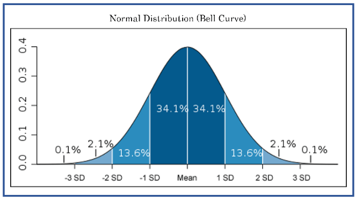
That is life! It’s known as the Regular Distribution or Bell Curve. It exhibits how far-off from the common most bodily and statistical issues are. Issues like folks’s heights or the variety of hurricanes in a decade.
We use the Regular Distribution to check the null speculation, the declare that there isn’t a “statistically important” distinction between the common and what we truly observe. More often than not, 68 % of the time, observations are near the common, inside one normal deviation – the common distance of the information from the common itself. As you progress farther from the common, you get much less of no matter it’s you’re counting. There are much more six-foot guys than seven-foot guys.
 Slide 2A
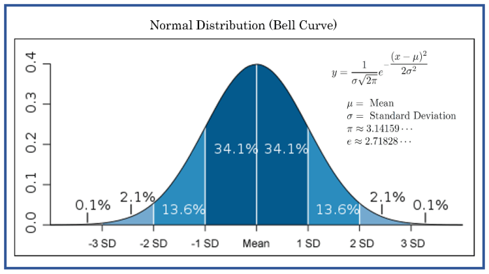
This components, derived from our arithmetic and amazingly confirmed in nature, determines the peak of the Regular curve at each level. It tells us simply how typically what we observe will likely be, just by likelihood, a sure variety of normal deviations away from the common.
 Slide 2B
This “Z-table” tells you precisely, to the third decimal place, how possible it’s that an statement occurred by likelihood. Once we run an experiment, we solely reject the null speculation, and say there’s a statistically important correlation, if the end result would occurred anyway one day trip of 20, or 5 % of the time. That makes us 95 % certain that the 2 variables are correlated, or transfer collectively.
 Slide 2C
Now, correlation just isn’t essentially causation. Life just isn’t bivariate – based mostly on simply the 2 issues you’re measuring. Until you may randomly assign topics, life is multivariate, with different variables inflicting modifications too. That is the commonest error in public coverage. In Latin it’s known as submit hoc ergo propter hoc: this factor occurred after that factor, so it was attributable to it. Right here’s an instance.
 Slide three – Scouting and Delinquency
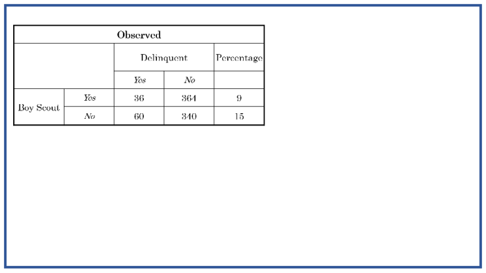
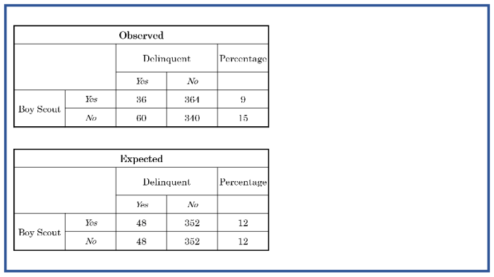
Does being a Boy Scout hold you out of hassle? Fast, maintain a press convention: solely 9 % of scouts are delinquents, versus 15 % of non-scouts.
 Slide 3A
The likelihood of getting such an enormous distinction from the null expectation of no distinction at 12 % is …
 Slide 3B
… lower than one %. You’ll be able to see that within the column labeled “Likelihood?” zero.009 is lower than zero.01, which is one %. Scouting works!
 Slide four – Subgroups
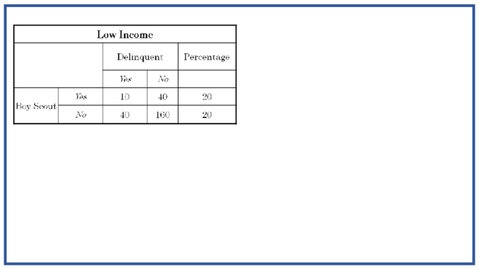
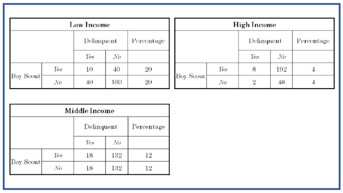
Now let’s management for one more vital variable in life, a household’s earnings degree. However this slide exhibits that there isn’t a distinction within the low-income households in delinquency charges for Scouts and non-Scouts; each are at 20 %.
 Slide 4A
And in middle-income households, once more no distinction, at 12 %. I suppose all of the distinction in delinquency should come from the high-income households.
 Slide 4B
Huh? No distinction right here both, with each teams at 4 % delinquency.
 Slide 4C
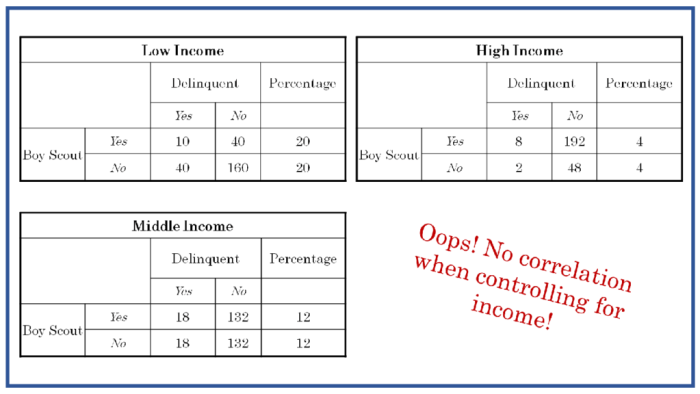
So, oops, the correlation disappears when controlling for earnings, which in contrast to scouting, is actually correlated with arrests.
 Slide 5 – Developments in Crime
One other method that correlation is confused with causation is in pattern strains. You see the drop in violent crime in a metropolis. The mayor, in fact, calls a press convention to take credit score.
 Slide 5A
Everyone has their very own clarification.
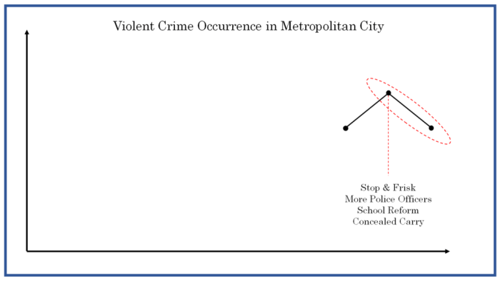 Slide 5B
However they agree one thing prompted the drop to occur.
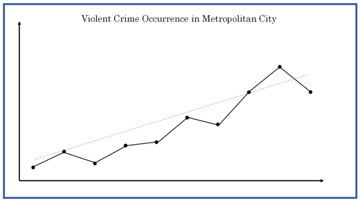 Slide 5C
A rising pattern line appears to say so.
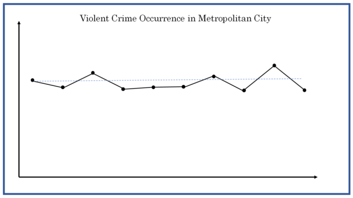 Slide 5D
However a flat pattern line …
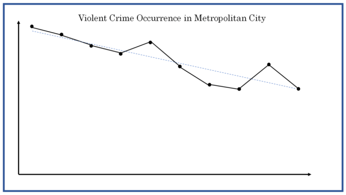 Slide 5E
… or a falling line would appear to point that it’s all simply random fluctuations. Cancel the press convention.
However the level right here is that NONE of this stuff we’re seeing with our eyes have ANY proof in them. A easy bivariate chart is inherently deceptive. All these graphs are literally worse than ineffective, as a result of they trick folks into considering they aren’t!
 Slide 6 – Sea Ranges
Let’s apply what we’ve discovered to “local weather change.” Take sea-level. There weren’t sufficient emissions for CO2 to be an element till 1950, so we evaluate the speed of sea-level rise earlier than and after 1950, and see if it has elevated.
However the United Nations Worldwide Panel on Local weather Change agrees that the distinction within the two slopes isn’t statistically important. No “local weather change.” [See Testimony of Caleb S. Rossiter, Ph.D. before the Subcommittee on the Environment of the House Committee on Oversight and Reform]
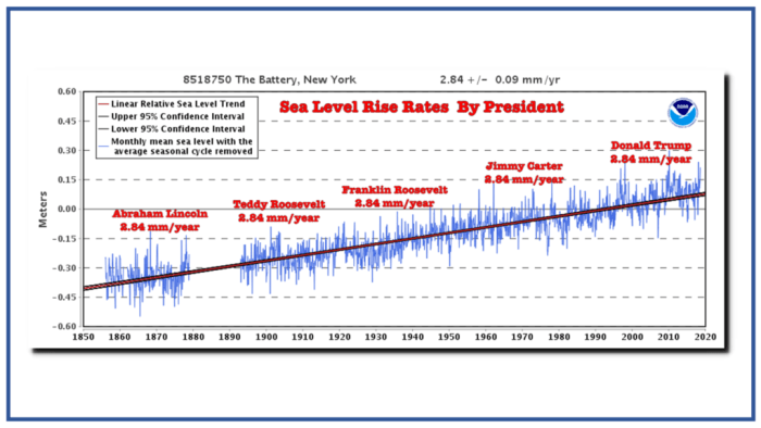 Slide 7 – Sea Degree by Presidents
Right here’s a enjoyable method to take a look at the identical type of knowledge: sea-level has truly been rising because the 1800’s after the Little Ice Age ended, on the identical price for all types of presidents and ranges of emissions!
 Slide eight – Hurricanes
How about hurricanes? In the event you simply take a look at the pattern from 1970 to 2010, you’d see an increase. However from 1940 to 2010, you’d see a drop. And from 1850 to 2010, you’d see no pattern in any respect. It’s the identical for floods, wildfires, and droughts: no long-term, statistically important will increase from the CO2 impact. “Detection and Attribution” research declare to detect an increase in some excessive climate variable like hurricanes after which they attribute that rise to elevated temperature from human exercise. These research lie within the realm of politics, not science, as a result of there’s no method to inform if the rise in temperature was pure or based mostly on industrial emissions.
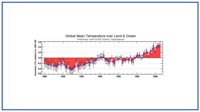 Slide 9 – International Imply Floor Temperature
And talking of temperature, right here is an iconic however deceptive UN IPCC graph. It exhibits the common change in temperature at floor stations, together with uncertainty and a long-term pattern line, in blue.
There’s a half diploma rise from 1910 to 1940, a flat interval till 1980, after which one other half diploma rise to 2010. With CO2 ranges barely rising till 1950, after which zooming up since then, that’s a whole lot of variation that’s not defined by CO2 emissions. Chaos, pure fluctuation, and unknown or arduous to quantify cycles are all a part of this image.
What’s so deceptive? First, it’s arduous to estimate a worldwide and even native common temperature in tenths of a level. You’ll be able to see that by the uncertainty, which itself is a guess. Floor temperature stations are problematic, not simply in 1880 however at present. Second, the information from many years in the past are consistently being adjusted with new guidelines to indicate extra rise.
 Slide 9A
We actually needs to be taking a look at international floor temperature at present, not to mention in 1900, on a scale of levels reasonably than tenths, like right here. These are the very same knowledge. Onerous to see a pattern in any respect.
 Slide 9B
Satellite tv for pc and balloon readings of the troposphere are rather more credible than the floor knowledge, however they’ve solely been gathered since 1980, so we are able to’t use them for longer developments.
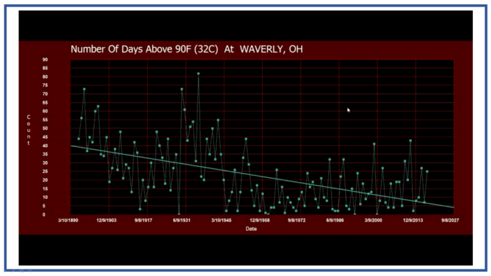 Slide 10 – Heat days in Ohio
Right here’s a typical temperature trick, courtesy of Tony Heller. The variety of days per yr over 90 levels on this city has been reducing from 1890 to 2017. Tony exhibits us tips on how to reverse that.
 Slide 10A
He strikes the beginning till you may declare a rise! At 1955 you get the “local weather change” graph you want. This type of deceptive purchasing for a begin date is usually performed in UN and U.S. local weather studies. [See U.S. Government Climate Science vs. U. S. Government Climate Crisis]
 Slide 11 – CO2 and Temperature
Right here’s a well-known UN slide of carbon dioxide and Antarctic temperature from ice cores.
 Slide 11A
Nicely, the slide grew to become notorious when Albert Gore Jr. gave us “correlation means causation”at its worst. Vice President Gore says CO2 drives temperature, however it’s largely the opposite method round: prolonged cycles in earth’s orbit change the Solar’s influence and drive temperature, which drives CO2. Gore hops on a riser to persuade us that as CO2 retains going up from industrial emissions, it’ll drag temperature alongside.
 Slide 11B
That prediction is already false, since temperature has barely budged on this scale.
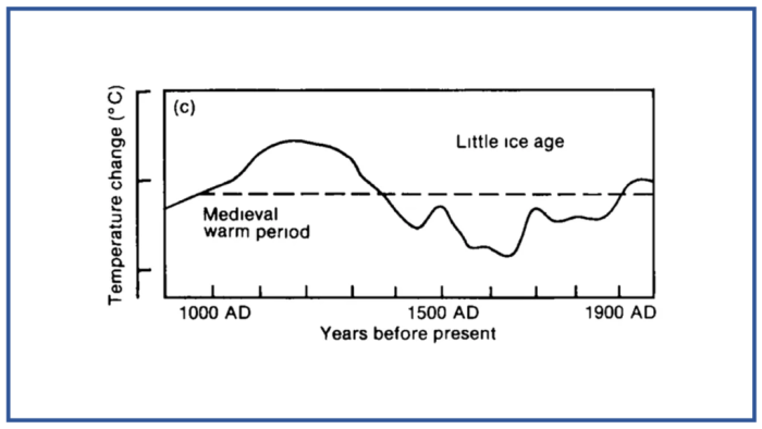 Slide 12 – A Thousand Years of Temperature
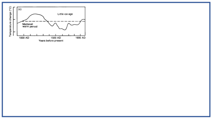
Now, is it hotter now than any time previously 1,000 years? It’s a foolish query, due to minimal protection for outdated knowledge. However even when the reply have been to be sure, it wouldn’t show something about what prompted the current rise. We now have a whole lot of the “hottest years on document” just lately solely as a result of the document is only one hundred years outdated and we occur to be in a interval of slight pure warming. That began in about 1800, properly earlier than the CO2 period. After all, throughout warming newer years are typically hotter than earlier years!
This graph appeared within the first UN report on local weather change, in 1990. It represents a reconstruction by local weather historians from diaries and proxies of what was roughly taking place to the globe. It goes up a few diploma in a Medieval Heat Interval and down a few diploma within the Little Ice Age, after which again up once more as that ended, all from pure causes. Many within the public claimed that the picture was embarrassing to the “local weather change” narrative.
 Slide 12A
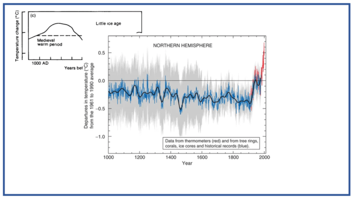
Somewhat than attempt to educate the general public about why this bivariate graph has no bearing by any means on what has prompted our current multivariate warming, the local weather change institution determined that the graph needed to go, and in 2001’s UN report, it did.
 Slide 12B
Rather than Medieval warming we bought a “hockey stick” with the blade rising solely within the industrial period. Temperature, it appears, was naturally fixed till dangerous fossil fuels got here alongside.
Now, for all of the inventive math utilized in creating this chart from just a few tree rings, it’s no higher or extra sure than the earlier, hand-drawn one.
 Slide 12C
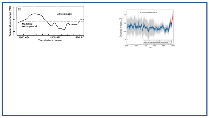
And I’ll present you why.
 Slide 12D
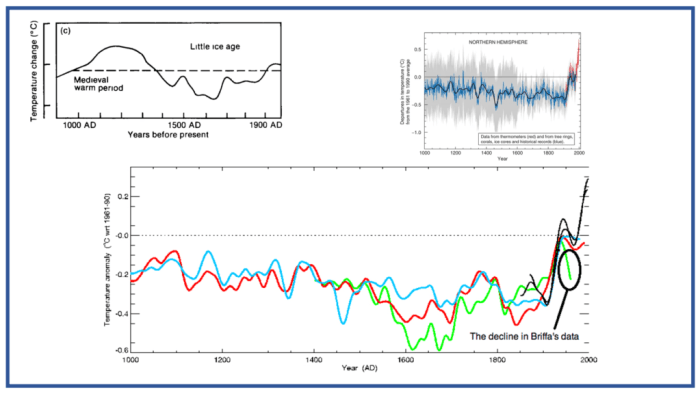
A key UN proxy set estimated by a researcher named Briffa exhibits that lately, temperatures calculated from tree rings go down, whereas we all know temperature was rising. Somewhat than rethink utilizing tree rings in any respect, the UN crowd – as revealed by their very own emails within the Climategate scandal – simply threw out the current knowledge to “cover the decline.”
We now have a saying about complicated calculations that depend on unsure knowledge: Rubbish in, rubbish out.
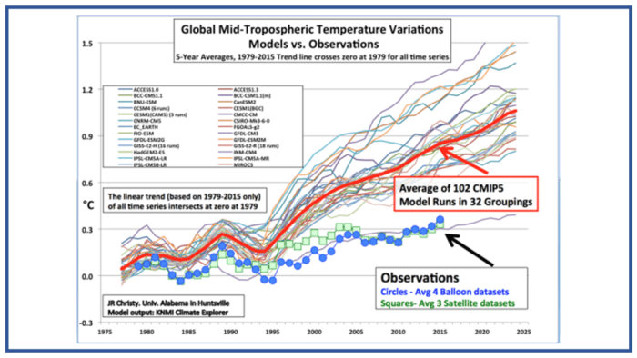 Slide 13 – Local weather Fashions
Talking of issues with knowledge and calculations, let’s finish with the mathematical pc fashions that drive the talk about harmful warming. International Local weather Fashions are based mostly on the Basic Circulation Fashions that predict native climate situations in your TV each night time. Climate fashions begin with wonderful native knowledge on situations and take a look at chances based mostly on earlier, precise climate in such situations. For just a few days then they will make an informed native guess.
The worldwide fashions, although, use common knowledge for very massive blocks of air, land, and sea, then add in carbon dioxide emissions and run for many years into the long run, the place there will be no comparability to precise situations. The fashions additionally use hundreds of estimates, known as parameters, to signify with only one quantity the impact of many complicated and chaotic bodily processes, just like the Hadley cells, wind techniques that transfer warmth from the decrease latitudes to the poles.
Legendary physicist Freeman Dyson dismissed such parameters as “fudge components.” They’re all simply guesses, just like the Medieval warming graph, that are twiddled and tweaked till the temperature output in previous many years is “tuned” to match the floor temperature document then.
Now, in fact, the floor document goes to be fallacious at the beginning – it’s a tough estimate itself – and the parameters are additionally going to be fallacious as properly– they’re guesses. What a multitude! After which the true parameters will change each cyclically and chaotically because the mannequin is run into the long run, however the modeled parameters is not going to. Yikes!
The essential output of those fashions is an estimate of “local weather sensitivity” – the levels of warming we’ll get from a doubling of CO2 – however that’s utterly decided by the modeler’s selection of the enter parameter for the way highly effective CO2 molecules are at warming! Loopy … however true. Just like the hockey stick, this seems to be a waste of time. Once more, how do we all know?
Nicely, first we are able to take a look at these fashions in opposition to their very own projections, and these constantly run about 3 times too sizzling over the previous 30 years. So the modelers consistently should “retune” the parameters and undertaking the long run another time.
However this graph right here can’t be tuned away, as a result of it checks even the up-to-date floor fashions in opposition to their projections within the troposphere, as much as about 40,000 ft, the place they are often checked by the much better satellite tv for pc and balloon readings. Have a look: the fashions’ projections for the troposphere, the thick pink line, additionally run 3 times too sizzling in comparison with precise temperatures, the road purple line, proper now, with out even ready for the long run.
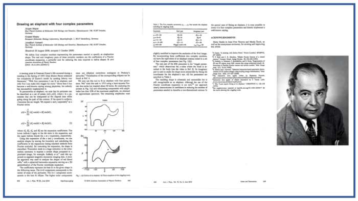 Slide 14 – The Elephant Paper
You’ll be able to perceive fashions’ weaknesses from a cautionary story about an elephant. John von Neumann was a legendary mathematician and atomic bomb maker who tried to construct a local weather mannequin after World Struggle II. He needed to make use of it as a weapon, to create a drought within the Soviet Union.
When von Neumann gave up, he laughed that: “With 4 parameters I can match an elephant, and with 5 I could make him wiggle his trunk.” Just lately, although, three mathematicians wrote this paper displaying the way it might be performed with capabilities of complicated numbers. See https://publications.mpi-cbg.de/Mayer_2010_4314.pdf
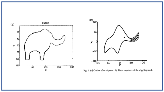 Slide 15 – The Elephant
The primary 4 capabilities draw the elephant on the left. Then, within the graph on the precise, a fifth parameter is added and adjusted, giving us some completely different placements of the trunk…it wiggles, as required! The purpose right here is that mathematical local weather fashions are managed by their hundreds of handy selections of parameters, and you may make these parameters do something you need. And since fashions can’t be examined statistically, all we’re left with once more is artwork, not science.
 Slide 16 – Questions
Nicely, that is Professor Caleb Rossiter, and I hope you’ve gotten thought quite a bit and discovered at the very least a bit of with this lecture on Local weather Statistics 101. Please be happy to contact me with any questions or feedback, at information@co2coalition.org.
Like this:
Loading…