How error propagation works with differential equations (and GCMs)
visitor publish by Nick Stokes
There was a whole lot of dialogue currently of error propagation in local weather fashions, eg right here and right here. I’ve spent a lot of my skilled life in computational fluid dynamics, coping with precisely that drawback. GCM’s are a particular sort of CFD, and each are functions of the numerical answer of differential equations (DEs). Propagation of error in DE’s is a central concern. It’s often described below the heading of instability, which is what occurs when errors develop quickly, often as a result of a design fault in this system.
So first I ought to say what error means right here. It’s only a discrepancy between a quantity that arises within the calculation, and what you imagine is the true quantity. It doesn’t matter for DE answer why you suppose it’s unsuitable; all that issues is what the iterative calculation then does with the distinction. That’s the propagation of error.
A normal linear equation in time could be formulated as
y’ = A(t)*y+f(t) ……….(1)
y(t) might be only one variable or a big vector (as in GCMs); A(t) might be a corresponding matrix, and f(t) might be some exterior driver, or a set of perturbations (error). The y’ means time spinoff. With a non-linear system corresponding to Navier-Stokes, A might be a operate of y, however this dependence is small regionally (in house and time) for a area; the fundamentals of error propagation comply with from the linearised model.
I’ll begin with some bits of DE idea which you could skip (I’ll get extra particular quickly). When you have one other answer z which is the answer following an error, then the distinction satisfies
(y-z)’=A*(y-z)
The dependence on f(t) has gone. Error propagation is decided by the homogeneous half y’=A*y.
You possibly can write down the options of this equation explicitly:
y(t) = W(t)*a, W(t) = exp(∫ A(u) du )
the place the exp() is generally a matrix exponential, and the integral is from beginning time zero to t. Then a is a vector representing the preliminary state, the place the error will seem, and the exponential determines how it’s propagated.
You will get a good distance by simply analysing a single error, as a result of the system is linear and situations could be added (superposed). However what if there’s a string of sequential errors? That corresponds to the unique inhomogeneous equation, the place f(t) is a few sort of random variable. So then we want an answer of the inhomogeneous equation. That is
y(t) = W(t) ∫ W-1(u) f(u) du, the place W(t)=exp(∫ A(v) dv ), and integrals are from zero to t
To get the overall answer, you may add any answer of the homogeneous equation.
For the actual case the place A=zero, W is the id, and the answer is a random stroll. However solely in that exact case. Typically, it’s one thing very completely different. I’ll describe some particular instances, in a single or few variable. In every case I present a plot with an answer in black, a perturbed answer in crimson, and some random options in pale gray for context.
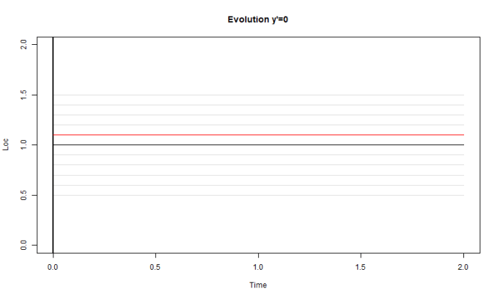
Particular case 1: y’=zero

That is the only differential equation you may have. It says no change; every part stays fixed. Each error you make continues within the answer, however doesn’t develop or shrink. It’s of curiosity, although, in that if you happen to maintain making errors, the result’s a random stroll.
Particular case 2: y”=zero

The case of no acceleration. Now if there may be an error within the velocity, the error in location will continue to grow. Already completely different, and already the straightforward random stroll answer for successive errors doesn’t work. The steps of the stroll would broaden with time.
Particular case three: y’=c*y
the place c is a continuing. If c>zero, the options are rising exponentials. The errors are additionally options, so that they develop exponentially. It is a case crucial to DE observe, as a result of it’s the mode of instability. For actually linear equations the errors improve in proportion to the answer, and so perhaps don’t matter a lot. However for CFD it’s often a blow-up.
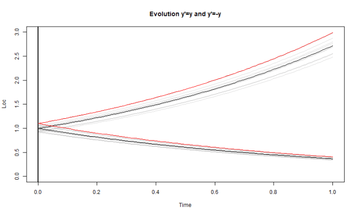
However there are simplifications, too. For the case of steady errors, the sooner ones have grown lots by the point the later ones get began, and actually are the one ones that rely. So it loses the character of random stroll, due to the skewed weighting.
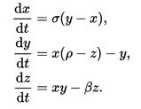
If c This particular case is essential, as a result of it corresponds to the behaviour of eigenvalues within the normal answer matrix W. A single constructive eigenvalue of A can produce rising options which, began from any error, will develop and develop into dominant. Conversely the various options that correspond to damaging eigenvalues will diminish and don’t have any persevering with impact. Simply taking a look at linear equations offers an oversimplified view the place errors and options change in proportion. The options of this equation are the features tanh(t+a) and coth(t+a), for arbitrary a. They have an inclination to 1 as t→∞ and to -1 as t→-∞. Convergence is exponential. So an error made close to t=-1 will develop quickly for some time, then plateau, then diminish, ultimately quickly and to zero. That is the poster little one for vigorous error propagation. It results in chaos, which I’ll say extra about. However there’s a lot to be learnt from evaluation. I’ve written in regards to the Lorenz attractor right here and in posts linked there. At that hyperlink you may see a gadget that may can help you generate trajectories from arbitrary begin factors and end occasions, and to see the leads to 3D utilizing webGL. A typical view is like this Lorenz derived his equations to signify a quite simple local weather mannequin. They’re: The parameters are conventionally σ=10, β=eight/three, ρ=28. My view above is within the x-z aircraft and emphasises symmetry. There are three stationary factors of the equations, 1 at (zero,zero,zero),(a, a, 27)and,(-a, -a, 27) the place a = sqrt(72). The final two are centres of the wings. Close to the centres, the equations linearise to present an answer which is a logarithmic spiral. You possibly can consider it as a model of y’=a*y, the place a is complicated with small constructive actual half. So trajectories spiral outward, and at this stage errors will propagate with exponential improve. I’ve proven the trajectories on the plot with rainbow colours, so you may see the place the bands repeat, and the way the colours steadily separate from one another. Paths close to the wing however not on it are drawn quickly towards the wing. Because the paths transfer away from the centres, the linear relation erodes, however actually fails approaching z=zero. Then the paths move round that axis, additionally dipping in direction of z=zero. This brings them into the area of attraction of the opposite wing, and so they drop onto it. That is the place a lot mixing happens, as a result of paths that had been solely reasonably far aside fall onto very completely different bands of the log spiral of that wing. If one falls nearer to the centre than the opposite, it will likely be a number of laps behind, and worse, velocities drop to zero towards the centre. As soon as on the opposite wing, paths steadily spiral outward towards z=zero, and repeat. Is the Pope Catholic? you would possibly ask. However chaos just isn’t dangerous, and we dwell with it on a regular basis. There’s a whole lot of construction to the Lorenz attractor, and if you happen to noticed a complete lot of random factors and paths sorting themselves out into this form, I feel you’ll marvel not on the chaos however the order. Actually we take care of info within the absence of answer paths on a regular basis. A store features completely properly despite the fact that it may’t hint which cash got here from which buyer. Extra scientifically, consider a cylinder of gasoline molecules. Computationally, it’s unattainable to comply with their paths. However we all know lots about gasoline behaviour, and might design environment friendly ICE’s, for instance, with out monitoring molecules. Actually, we will infer virtually every part we need to know from statistical mechanics that began with Maxwell/Boltzmann. CFD embodies chaos, and it’s a part of the way in which it really works. Individuals usually consider turbulence there, however it might be chaotic even with out it. CFD options rapidly lose detailed reminiscence of preliminary circumstances, however that could be a constructive, as a result of in sensible circulate we by no means knew them anyway. Actual circulate has the identical function as its computational analogue, as one would want. If it did rely on preliminary circumstances that we might by no means know, that may be an issue. So that you would possibly do wind tunnel checks to find out elevate and drag of a wing design. You by no means know preliminary circumstances in tunnel or in flight nevertheless it doesn’t matter. In CFD you’d begin with preliminary circumstances, however they quickly get forgotten. Simply as properly. GCMs are CFD and in addition can not monitor paths. The identical lack of preliminary info happens on one other scale. GCMs, working as climate forecasts, can monitor the dimensions of issues we name climate for just a few days, however not additional, for basically the identical causes. However, like CFD, they’ll generate long term options that signify the response to the steadiness of mass, momentum and power over the identical long term. These are the local weather options. Simply as we will have a gasoline regulation which supplies bulk properties of molecules that transfer in methods we will’t predict, so GCMs give details about local weather with climate we will’t predict. Evaluation of error in CFD and GCMs is generally performed to design for stability. It will get too sophisticated for quantitative tracing of error, and so a extra rigorous and complete answer is used, which is … simply do it. If you wish to know the way a system responds to error, make one and see. In CFD, the place a serious supply of error is the spatial discretisation, a typical method is to seek for grid invariance. That’s, remedy with finer grids till refinement makes no distinction. With climate forecasting, a regular methodology is use of ensembles. If you’re uncertain of enter values, strive a spread and see what vary of output you get. And that is performed with GCMs. In fact there the runs are costlier, and to allow them to’t do a full vary of variations with every run. Alternatively, GCM’s are usually surveying the identical local weather future with simply completely different situations. So any average diploma of ensemble use will accumulate the required info. One other factor to recollect about ensemble use in GCM’s is that this. You don’t have to fret about testing one million completely different attainable errors. The reason being associated to the lack of preliminary info. In a short time one error begins to look just about like one other. That is the filtering that outcomes from the fluctuate giant eigenspace of modes which can be damped by viscosity and different diffusion. It is just the impact of error on a fairly small house of attainable options that issues. When you take a look at the KNMI CMIP 5 desk of GCM outcomes, you’ll see a complete lot of fashions, situations and consequence varieties. However if you happen to take a look at the small quantity beside every radio button, it’s the ensemble vary. Typically it’s only one – you don’t should do an ensemble in each case. However fairly often it’s 5,6 and even 10, only for 1 program. CMIP has a particular notation for recording whether or not the ensembles are various simply preliminary circumstances or some parameter. Error propagation is essential in differential equations, and could be very a lot a property of the equation. You possibly can’t analyse with out taking that into consideration. Quick rising errors are the primary explanation for instability, and have to be attended to. The easiest way to check error propagation, if computing sources are enough, is by an ensemble methodology, the place a spread of perturbations are made. That is performed with earth fashions, each forecasting and local weather. One criticised function of Pat Frank’s paper was the usage of a simplified equation (1) which was subjected to error evaluation instead of the extra complicated GCMs. The justification given was that it emulated GCM options (really a mean). Is that this OK? Given an answer f(t) of a GCM, you may really emulate it completely with an enormous number of DEs. For any coefficient matrix A(t), the equation y’ = A*y + f’ – A*f has y=f as an answer. An ideal emulator. However as I confirmed above, the error propagation is given by the homogeneous half y’ = A*y. And that might be something in any respect, relying on alternative of A. Sharing a typical answer doesn’t imply that two equations share error propagation. So it’s not OK. Loading…
Particular case four: Non-linear y’=1-y2

Particular case 5: the Lorenz butterfly

Is chaos dangerous?
GCMs and chaos
What is completed in observe? Ensembles!
Conclusion
Appendix – emulating GCMs
Like this: