Fashions, Feedbacks, And Propagation Of Error

Visitor put up by Kevin Kilty

Introduction

I had contemplated a contribution involving suggestions diagrams, techniques of equations, differential equations, and propagation of error ever since Nick Stoke’s authentic contribution a couple of system of differential equations involving suggestions method again in June of this 12 months. A few days in the past the person Bartemis posted a pair of differential equations in a put up of Roy Spencer which offered some inspiration on tying all these ideas collectively in a single posting. Lastly, an added inspiration got here from the controversy about Pat Frank’s current contribution. With out taking a stand on the numerical values Pat calculated, or his strategy, I hope to reveal why he and his critics, Nick for instance, are actually discussing various things; and why Pat’s tackle this matter deserves very cautious consideration. Right here goes.

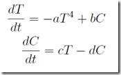
Let’s think about the next system of equations:

(1)

(2)

We are able to view this as a mannequin of water vapor suggestions the place; T is a floor temperature, C is a focus of water vapor, and a,b,c,d are constants. The set of equations is a system of first order differential equations, however non-linear. One can even view particular person phrases as second order if we differentiate the primary equation, and substitute into it the second. As an illustration, within the instance of temperature (T):

(three)

This, too, is non-linear however now a second order differential equation.

Thus, we will have a look at the temperature downside as a part of a primary order

system, or as a second order differential equation. It doesn’t matter besides that the primary order system is simpler to take care of mathematically.

1. Making a linear approximation

The system of equations has two regular options, which an individual can confirm by easy substitution. These are (T0 = zero, C0 = zero) or (T0 = (bc/da)1/three , C0 = c/d · T0). The primary is a trivial resolution of no curiosity. The second turns into some extent round which we’ll make a linear approximation to the unique equation set. The algebra is slightly tedious and has little bearing on the problems at hand. But when we name ζ a small deviation from the regular resolution in water vapor, and θ a small deviation in temperature the ultimate type of the set of equations is.

(four)

(5)

These are legitimate close to the stationary resolution (T0 = (bc/da)1/three , C0 = c/d·T0). Doing as we did to supply the second order Equation three) we arrive on the following linear second order approximation.

(6)

2. Suggestions Block Diagrams

Earlier than persevering with towards my predominant function, I’d like to indicate the connection of the differential equations, above, to suggestions diagrams over which individuals have spilled electrons galore, though solely inexperienced ones, on these pages. Figures 1a and 1b present two doable block fashions of the second order differential equation in θ. The block fashions, and the differential equations are simply completely different descriptions of the identical factor. One has no mojo that the opposite doesn’t have. They’ve completely different utility. For instance, engineers should flip a system into digital or mechanical that realizes the system, and the block diagram is beneficial for making this transformation.

Determine 1. Figures a, and b present various block fashions of the second order differential equation in θ. In a) the mannequin consists of two integrators, which flip θ¨ into θ, and the suggestions loops comprise acquire blocks. In b) there’s a filter that features as a leaky integrator. Block representations aren’t distinctive.

three. Stability of the Linear System

We’re able now to use Nick’s stability evaluation. Discovering the eigenvalues of a two by two matrix is comparatively straightforward. It simply makes use of the quadratic components. The reader may seek the advice of Wolfram Math World on-line (mathworld.wolfram.com/Eigenvalue.html) which exhibits eigenvalues on this occasion explicitly.

(7)

There are two unfavourable eigenvalues for some mixtures of (h,b,c,d), that means; the linearized system is steady, and the unique non-linear system is then steady towards infinitesimal disturbances. As Nick Stokes indicated, preliminary errors on this system will damp out. This, nevertheless, shouldn’t be the complete story. In my view it’s the appropriate reply to a unsuitable query. The query of stability isn’t just a matter of the habits of matrix A, the place:

but in addition the query of what happens with explicit enter to the system. In a steady system like we will state bounded enter produces a bounded output. That’s good to know, however bounded doesn’t reply the extra complicated query of whether or not the output is beneficial for a particular function. This can be a area that propagation of error addresses. It’s, I sense, the place Pat Frank was taking in his essay, and whereas I don’t converse for him, one can’t dismiss the significance of what he was attempting to do.

four. The Actual Concern of Error Propagation

Let’s return to the linearized system (Eqs. four and 5 ). The system actually doesn’t do a lot of something fascinating as a result of there’s nothing to drive it. We will need to have a vector of driving phrases, one involving the motive force of temperature, and presumably one to drive water vapor. With out this all the answer ever does is decay again to the regular resolution–i.e. its errors vanish. However this misses a number of essential issues. In design of management system, the engineer has to take care of inputs and disturbances to the system. Thus, the photo voltaic fixed varies barely and pushes the answer away from the equilibrium one.[1] We’d put this within the vector U in Equation eight). There are undoubtedly disturbances driving the quantity of water vapor as nicely. The subsequent degree of issue is having a mannequin that’s not totally specified. As an illustration, El Nino shouldn’t be a part of the state vector, but it surely does provide a disturbance to temperature and humidity. Thus it belongs in vector e in Equation eight). Maybe these lacking parameters present random influences which then seem to have come from the photo voltaic fixed or from water vapor. Lastly, by being solely a mannequin, we can’t presumably know true values of the matrix components of ; we estimate them finest we will, however they’re unsure.

A extra reasonable mannequin of what we’re coping with seems like this state house mannequin involving the vector of two state variables, temperature and humidity (X), and the drivers and random errors of enter (U + e). Simply to be full I’ve famous that what we observe shouldn’t be essentially the state variables, however fairly some perform of them which will have handed by means of devices first. What we observe is then another vector, Y, which could have its personal added errors, w, fully unbiased of errors added to the drivers.

(eight) X˙ = · X + · (U + e)

(9) Y = C · X + · (U + w)

Though it’s a extra reasonable mannequin, it nonetheless doesn’t describe propagation of error, however its resolution is required equipment to get at propagated error. What we wish to estimate, utilizing an answer to those equations is an expectation of the distinction between what we might observe with a finest mannequin, which we will’t presumably know precisely, and what the mannequin equations above produce with uncertainties thought-about.

Here’s a regular resolution to our state variables: X = · U + e. The matrix comes from a mixture of the matrices and , the small print of which don’t matter right here.[2] As a matrix we will say merely that seems like this:

5. An Estimate of Uncertainty

There is no such thing as a function to turning into slowed down in extreme arithmetic. So, let‘s focus consideration on solely the equation for temperature, θ. It’s obvious that we do not need a whole or correct mannequin of temperature. Thus, let regardless of the equations eight) and 9) produce as an answer be known as an estimate of temperature. We use the image θˆ for this. The caret image is what statisticians typically use for an estimator. Then let the true temperature we might have discovered from an ideal mannequin be θ. Though we don’t really know the true θ we determine our mannequin shouldn’t be too dangerous and so θˆis close by regardless of uncertainties.

Usually individuals use a Taylor collection to construct a linear approximation to θˆ, and calculate error propagation from it. This Taylor collection is written by way of partial derivatives of all unsure unbiased variables and parameters, the pis, within the following.

(10)

However in our particular case the phrases of G, the gij, are coefficients of the linear approximation, with the drivers, the weather of the vector (U + e), as inputs. Thus our first order Taylor collection seems like:

(11) (θˆ− θ) = g11 · (u1 + e1) + g12 · (u2 + e2)

As an estimate of propagated error what we require is the variance of (θˆ−θ) as a result of, now having random enter, this distinction has grow to be a random variable itself. Variance is outlined usually as E((Z−E(Z))2); the place E(…) means expectation worth of the random variable inside the parentheses.[3] Due to this fact we must always sq. equation 11) and take the expectation worth, in order that what resides on the left hand facet is the expectation worth of variance we search. Name this Sθ2. The proper hand facet of equation 11) produces many phrases as there are unsure parameters, plus cross merchandise.

(12)

Sθ2 = g112 ·E[(u1+e1)2]+g122 ·E[(u2+e2)2]+2·g11g12·E[(u1+e1)·( u2+e2)]

The phrases inside sq. brackets are variances or covariances. Even when the expectation values of the random inputs are zero, their variances aren’t. Thus, regardless of having a steady system of differential equations, the variance of the state variables in all probability is not going to are likely to zero as time progresses.

There’s a additional level to debate. The matrix shouldn’t be identified precisely. Every ingredient has some uncertainty which equations eight) and 9) don’t point out explicitly. One solution to embrace that is to put a uncertainty matrix in collection with ; which then turns into + . is sort of a matrix of random variable which we assume have expectation values of zero for all components, however as soon as once more do not need zero variance. This matrix will produce uncertainty in , by means of its relationship to . An entire propagation of error takes some thought and care.

6. Conclusion

The worth of Sθ2 which ends from a whole evaluation of the contributors to uncertainty when in comparison with the precision wanted, is what actually determines whether or not or not mannequin outcomes are match for function. As I wrote in a remark at one level in Pat’s authentic posting, the subject of propagation of error is complicated; and I used to be informed that it’s certainly not complicated. I feel this dialogue exhibits that it’s extra complicated than many individuals suppose, and I hope it helps reinforce Pat Frank’s factors.

7. Notes:

(1) = ( −λ·I)−1 See, as an example, Ogata, System Dynamics, 2004, Pearson-Prentice Corridor.

(2) Mototaka Nakamura, in his current monograph, which is obtainable for obtain at Amazon.com, alludes to small variations within the photo voltaic fixed. This is able to go into the vector U for instance.

(three) That is defined nicely in Bevington, Knowledge Discount and Error Evaluation for the Bodily Sciences, McGraw-Hill, 1969. Bevington illustrates quite a few easy instances. Neither his, nor another reference I do know, tackles propagated error by means of a system of linear equations.

Like this:

Like Loading…