Critique of “Propagation of Error and the Reliability of World Air Temperature Predictions”
From Dr. Roy Spencer’s Weblog
September 11th, 2019 by Roy W. Spencer, Ph. D.
I’ve been requested for my opinion by a number of folks about this new printed paper by Stanford researcher Dr. Patrick Frank.
I’ve spent a few days studying the paper, and programming his Eq. 1 (a easy “emulation mannequin” of local weather mannequin output ), and included his error propagation time period (Eq. 6) to ensure I perceive his calculations.
Frank has supplied the quite a few peer reviewers’ feedback on-line, which I’ve purposely not learn with a view to present an unbiased evaluate. However I principally agree along with his criticism of the peer evaluate course of in his latest WUWT submit the place he describes the paper in easy phrases. In my expertise, “local weather consensus” reviewers typically give probably the most inane and irrelevant objections to a paper in the event that they see that the paper’s conclusion in any means may diminish the Local weather Disaster™.
Some reviewers don’t even learn the paper, they only have a look at the conclusions, see who the authors are, and decide primarily based upon their preconceptions.
Readers right here know I’m important of local weather fashions within the sense they’re getting used to supply biased outcomes for power coverage and monetary causes, and their elementary uncertainties have been swept beneath the rug. What follows just isn’t meant to defend present local weather mannequin projections of future world warming; it’s meant to point out that — so far as I can inform — Dr. Frank’s methodology can’t be used to show what he thinks he has demonstrated in regards to the errors inherent in local weather mannequin projection of future world temperatures.
A Very Temporary Abstract of What Causes a World-Common Temperature Change
Earlier than we go any additional, you will need to perceive some of the primary ideas underpinning temperature calculations: With few exceptions, the temperature change in something, together with the local weather system, is because of an imbalance between power achieve and power loss by the system. That is primary 1st Legislation of Thermodynamics stuff.
So, if power loss is lower than power achieve, warming will happen. Within the case of the local weather system, the warming in flip ends in a rise lack of infrared radiation to outer area. The warming stops as soon as the temperature has risen to the purpose that the elevated lack of infrared (IR) radiation to to outer area (quantified via the Stefan-Boltzmann [S-B] equation) as soon as once more achieves world power stability with absorbed photo voltaic power.
Whereas the particular mechanisms may differ, these power achieve and loss ideas apply equally to the temperature of a pot of water warming on a range. Underneath a relentless low flame, the water temperature stabilizes as soon as the speed of power loss from the water and pot equals the speed of power achieve from the range.
The local weather stabilizing impact from the S-B equation (the so-called “Planck impact”) applies to Earth’s local weather system, Mars, Venus, and computerized local weather fashions’ simulations. Only for reference, the typical flows of power into and out of the Earth’s local weather system are estimated to be round 235-245 W/m2, however we don’t actually know for certain.
What Frank’s Paper Claims
Frank’s paper takes an instance recognized bias in a typical local weather mannequin’s longwave (infrared) cloud forcing (LWCF) and assumes that the everyday mannequin’s error (+/-Four W/m2) in LWCF will be utilized in his emulation mannequin equation, propagating the error ahead in time throughout his emulation mannequin’s integration. The outcome is a big (as a lot as 20 deg. C or extra) of ensuing spurious mannequin warming (or cooling) in future world common floor air temperature (GASAT).
He claims (I’m paraphrasing) that that is proof that the fashions are basically nugatory for projecting future temperatures, so long as such massive mannequin errors exist. This sounds affordable to many individuals. However, as I’ll clarify under, the methodology of utilizing recognized local weather mannequin errors on this style just isn’t legitimate.
First, although, a number of feedback. On the constructive facet, the paper is well-written, with in depth examples, and is well-referenced. I want all “skeptics” papers submitted for publication have been as professionally ready.
He has supplied greater than sufficient proof that the output of the typical local weather mannequin for GASAT at any given time will be approximated as simply an empirical fixed instances a measure of the amassed radiative forcing at the moment (his Eq. 1). He calls this his “emulation mannequin”, and his result’s unsurprising, and even anticipated. Since world warming in response to rising CO2 is the results of an imposed power imbalance (radiative forcing), it is sensible you might approximate the quantity of warming a local weather mannequin produces as simply being proportional to the overall radiative forcing over time.
Frank then goes via many printed examples of the recognized bias errors local weather fashions have, notably for clouds, when in comparison with satellite tv for pc measurements. The modelers are effectively conscious of those biases, which will be constructive or detrimental relying upon the mannequin. The errors present that (for instance) we don’t perceive clouds and the entire processes controlling their formation and dissipation from primary first bodily rules, in any other case all fashions would get very practically the identical cloud quantities.
However there are two elementary issues with Dr. Frank’s methodology.
Local weather Fashions Do NOT Have Substantial Errors of their TOA Internet Power Flux
If any local weather mannequin has as massive as a Four W/m2 bias in top-of-atmosphere (TOA) power flux, it will trigger substantial spurious warming or cooling. None of them do.
Why?
As a result of every of those fashions are already energy-balanced earlier than they’re run with rising greenhouse gases (GHGs), in order that they don’t have any inherent bias error to propogate.
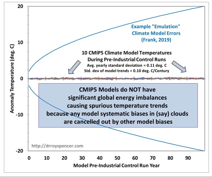
For instance, the next determine reveals 100 yr runs of 10 CMIP5 local weather fashions of their pre-industrial management runs. These management runs are made by modelers to be sure that there aren’t any long-term biases within the TOA power stability that might trigger spurious warming or cooling.
 Determine 1. Output of Dr. Frank’s emulation mannequin of world common floor air temperature change (his Eq. 1) with a +/- 2 W/m2 world radiative imbalance propagated ahead in time (utilizing his Eq. 6) (blue traces), versus the yearly temperature variations within the first 100 years of integration of the primary 10 fashions archived at
https://climexp.knmi.nl/selectfield_cmip5.cgi?id=somebody@someplace .
If what Dr. Frank is claiming was true, the 10 local weather fashions runs in Fig. 1 would present massive temperature departures as within the emulation mannequin, with massive spurious warming or cooling. However they don’t. You’ll be able to barely see the yearly temperature deviations, which common about +/-Zero.11 deg. C throughout the ten fashions.
Why don’t the local weather fashions present such habits?
The reason being that the +/-Four W/m2 bias error in LWCF assumed by Dr. Frank is nearly precisely cancelled by different biases within the local weather fashions that make up the top-of-atmosphere world radiative stability. It doesn’t matter how correlated or uncorrelated these numerous errors are with one another: they nonetheless sum to zero, which is why the local weather mannequin tendencies in Fig 1 are solely +/- Zero.10 C/Century… not +/- 20 deg. C/Century. That’s an element of 200 distinction.
This (first) downside with the paper’s methodology is, by itself, sufficient to conclude the paper’s methodology and ensuing conclusions will not be legitimate.
The Error Propagation Mannequin is Not Applicable for Local weather Fashions
The brand new (and usually unfamiliar) a part of his emulation mannequin is the inclusion of an “error propagation” time period (his Eq. 6). After introducing Eq. 6 he states,
“Equation 6 reveals that projection uncertainty should enhance in each simulation (time) step, as is predicted from the affect of a scientific error within the deployed idea“.
Whereas this error propagation mannequin may apply to some points, there isn’t a means that it applies to a local weather mannequin integration over time. If a mannequin really had a +Four W/m2 imbalance within the TOA power fluxes, that bias would stay comparatively fixed over time. It doesn’t in some way accumulate (because the blue curves point out in Fig. 1) because the sq. root of the summed squares of the error over time (his Eq. 6).
One other curious facet of Eq. 6 is that it’s going to produce wildly totally different outcomes relying upon the size of the assumed time step. Dr. Frank has chosen 1 yr because the time step (with a +/-Four W/m2 assumed power flux error), which can trigger a specific amount of error accumulation over 100 years. But when he had chosen a 1 month time step, there can be 12x as many error accumulations and a a lot bigger deduced mannequin error in projected temperature. This could not occur, as the ultimate error must be largely unbiased of the mannequin time step chosen. Moreover, the assumed error with a 1 month time step can be even bigger than +/-Four W/m2, which might have magnified the ultimate error after a 100 yr integrations much more. This makes no bodily sense.
I’m certain Dr. Frank is rather more professional within the error propagation mannequin than I’m. However I’m fairly certain that Eq. 6 doesn’t symbolize how a particular bias in a local weather mannequin’s power flux element would change over time. It’s one factor to invoke an equation which may effectively be correct and applicable for sure functions, however that equation is the results of a wide range of assumptions, and I’m fairly certain a number of of these assumptions will not be legitimate within the case of local weather mannequin integrations. I hope statistician corresponding to Dr. Ross McKitrick will study this paper, too.
Concluding Feedback
There are different, minor, points I’ve with the paper. Right here I’ve outlined the 2 most obvious ones.
Once more, I’m not defending the present CMIP5 local weather mannequin projections of future world temperatures. I consider they produce about twice as a lot world warming of the atmosphere-ocean system as they need to. Moreover, I don’t consider that they’ll but simulate recognized low-frequency oscillations within the local weather system (pure local weather change).
However within the context of world warming idea, I consider the most important mannequin errors are the results of a lack of information of the temperature dependent adjustments in clouds and precipitation effectivity (thus free-tropospheric vapor, thus water vapor “suggestions”) that truly happen in response to a long-term forcing of the system from rising carbon dioxide. I don’t consider it’s as a result of the basic local weather modeling framework just isn’t relevant to the local weather change challenge. The existence of a number of modeling facilities from world wide, after which performing a number of experiments with every local weather mannequin whereas making totally different assumptions, remains to be one of the best technique to get a deal with on how a lot future local weather change there *might* be.
My important criticism is that modelers are both misleading about, or unaware of, the uncertainties within the myriad assumptions — each express and implicit — which have gone into these fashions.
There are a lot of ways in which local weather fashions will be faulted. I don’t consider that the present paper represents certainly one of them.
I’d be glad to be proved unsuitable.
Like this:
Loading…